Professional data scientists know that data must be prepared before feeding any model with it. Data pre-processing is probably the most important part of a machine learning pipeline and its importance is sometimes underestimated.
Power transformations are a set of transformations that are very useful in certain situations. Let’s see when.
What is power transform?
Power transfom is a family of functions that transform data using power laws. The idea is to apply a transformation to each feature of our dataset.
What’s the purpose of a power transform? The idea is to increase the symmetry of the distribution of the features. If a features is asymmetric, applying a power transformation will make it more symmetric.
Let’s see an example using the breast cancer dataset in scikit-learn. If we draw the histogram of the first 6 features, we see that they are very asymmetric.
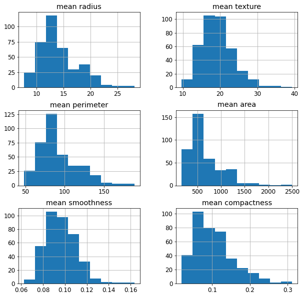
Some models may not work properly if the features are not symmetric. For example, models based on distances like KNN or K-means may fail if the distributions are skewed. In order to make these models work, power transformations will symmetrize the features without affecting their predictive power too much.
Some power transformations
The most common power transformations are the Box-Cox and the Yeo-Johnson transformations.
Box-Cox transformation has this formula:
{\displaystyle y ={\begin{cases}{\dfrac {y^{\lambda }-1}{\lambda }}&{\text{if }}\lambda \neq 0,\\\ln y&{\text{if }}\lambda =0,\end{cases}}}As you can see, we have a λ parameter that can be estimated using maximum likelihood. For example, we can try to minimize the skewness keeping the variance as stable as possible.
This formula must be applied to each feature independently. Each feature may potentially have different values for λ.
Since the independent variable appears inside a logarithm, this transformation can be applied only to strictly positive features.
If we apply the Box-Cox transformation to the previous dataset, we get:
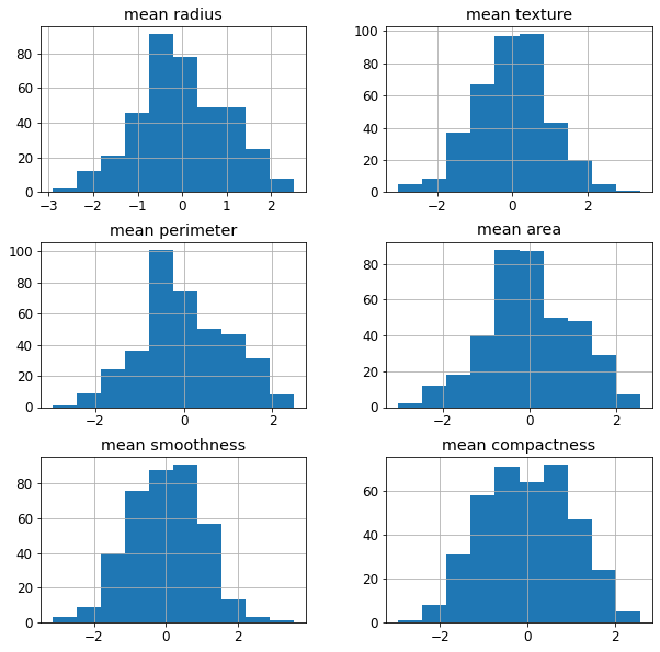
As you can see, the new features are more symmetric then the original ones.
Yeo-Johnson transformation has this formula:
{\displaystyle y={\begin{cases}((y+1)^{\lambda }-1)/\lambda &{\text{if }}\lambda \neq 0,y\geq 0\\\log(y+1)&{\text{if }}\lambda =0,y\geq 0\\-[(-y+1)^{(2-\lambda )}-1]/(2-\lambda )&{\text{if }}\lambda \neq 2,y<0\\-\log(-y+1)&{\text{if }}\lambda =2,y<0\end{cases}}}We still have a λ parameter to be estimated, but now this transformation can be applied even to negative features.
The result to our dataset is:
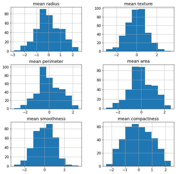
Again, we have a set of symmetric features that can be used by our model.
When to use power transformations
According to my experience, it’worth using power transformations when we use models based on distances like KNN, K-means, DBSCAN. Somebody says that they are useful with linear models and gaussian Naive Bayes, but I’m more sure about the former than the latter. Models based on trees and neural networks are not effected by the symmetry of the features, while SVM may sometimes need a power transformation in advance if we need to work only with linear kernels.
An example in python
Let’s see how to use power transformation in Python. We are going to use a KNN classifier on breast cancer dataset and see that using power transform will increase the performance of the model, that is measured using AUROC.
This code can be found in my GitHub repository here.
Let’s first import some libraries.
from sklearn.datasets import load_breast_cancer
import pandas as pd
from sklearn.preprocessing import StandardScaler
from sklearn.neighbors import KNeighborsClassifier
from sklearn.pipeline import Pipeline
from sklearn.metrics import roc_auc_score,balanced_accuracy_score
from sklearn.model_selection import GridSearchCV, train_test_split
from sklearn.preprocessing import PowerTransformer
import matplotlib.pyplot as plt
Let’s import the first 6 features of the dataset and store them into a pandas dataframe for simplicity.
d = load_breast_cancer()

df = pd.DataFrame(d['data'],columns=d['feature_names']).iloc[:,0:6]
We can now split this dataset into training and test.
X_train, X_test, y_train, y_test = train_test_split(df, d['target'], test_size=0.33, random_state=42)Now we can train our model on the training set and test it on the test set. We’re going to use the pipeline object in scikit-learn in order to apply the necessary feature scaling. For this first example, we are going to avoid the use of power transformations
model = Pipeline([
                  ('scaler',StandardScaler()),
                  ('model',KNeighborsClassifier())
])

model.fit(X_train,y_train)

roc_auc_score(y_test,model.predict_proba(X_test)[:,1])
Without power transform, we get an AUROC value equal to 0.976
Now, let’s try to use the power transformation. In Python, we have the PowerTransformer object, that performs Yeo-Johnson transform by default and searches for the best value of lambda automatically. We could use Box-Cox-transform if we wanted to, but for this example we’re going to use the default settings. Scaling could be avoided because PowerTransformer standardizes the features automatically, but it’s always a good habit to explicitly use it.
If we apply power transform to the pipeline (before the scaler), the code is:
model = Pipeline([
                  ('power',PowerTransformer()),
                  ('scaler',StandardScaler()),
                  ('model',KNeighborsClassifier())
])

model.fit(X_train,y_train)

roc_auc_score(y_test,model.predict_proba(X_test)[:,1])
Using the power transformation, the AUROC value increases to 0.986. So, this model performs better than the model without power transformed features.
Conclusions
Power transformations are very useful when we have to deal with skewed features and our model is sensitive to the symmetry of the distributions. It’s important to remember to use them before any kind of scaling.

